MNIST: using raccoon to cluster handwritten digits

In this tutorial, we will attempt to build a hierarchy of clusters from the popular MNIST dataset using basic raccoon functionalities. In the last sections, we will use this hierarchy to build a k-NN classifier.

You can follow these steps as a template for the clustering analysis of any of your datasets. See the manual for more features and options.

Dataset

As a first step, we can use Keras (not required by raccoon) to download or the MNIST dataset, and subset it to speed up the whole process. We download both the data and their labels, although this clustering is fully unsupervised, we can use this information to validate the classes and their hierarchy.

import pandas as pd
from keras.datasets import mnist


n_samples = 25000
seed = 32

(x_train, y_train), (x_test, y_test) = mnist.load_data()
x_train = x_train.reshape(x_train.shape[0],x_train.shape[1]*x_train.shape[2])
input_df = pd.DataFrame(x_train).sample(n_samples,random_state=seed)
labels = pd.Series(y_train).sample(n_samples,random_state=seed)

we reformat the input and its labels into pandas object, the library can work with any array-like format, but pandas data frames will make our life easier. We also fix the random state seed for debugging purposes.

Iterative Clustering

As our input is ready to go, we can now use it to run our first iterative clustering instance. Details on all the flags available to the run function can be found in the manual, here we select some default values as explained in the following paragraphs.

import raccoon as rc

cluster_membership, tree = rc.cluster(input_df, lab=labels, dim=2, pop_cut=50,
                    filter_feat='t_sVD', optimizer='de', depop=25, deiter=25,
                    nei_factor=0.5, metric_clu='euclidean', metric_map='cosine',
                    out_path='./raccoon_outputs/', save_map=True)

this function will automatically take care of initializing the clustering object and run it for us, it just requires the selection of which kind of tools to use.

Here we input the data, followed by their labels. As mentioned above, the lab flag is optional and is only used to output scatter plots colour-coded according to the original labels, if any are present. It can help in the annotation of the clusters if full or partial information is available. Make sure that the labels have corresponding indices to the input data, or, if you are using an array-like format, make sure the order of your data points and labels are matching.

The dim parameter sets the dimensionality of the target space. As we go towards fewer and fewer dimensions, we start introducing artifacts (tears and deformations) in the embedding, but the cost to identify the clusters and compute the objective function also decreases, making the calculations more efficient. When choosing this parameter one should weigh accuracy against cost. Here, for demonstration purposes, we chose to reduce our space to only two dimensions. This also allows us to choose metric_clu='euclidean' as the metric for the identification of the clusters and speed up considerably the calculations. When working with higher dimensions, metrics that handle >2 dimensions better (e.g. 'cosine' distance) should be used instead. metric_map sets the metric used for the non-linear dimensionality reduction step and should be left as by default unless you know what you are doing.

Note: When working with higher-dimensionality embedding, the library will keep producing two-dimensional plots to help with a visual inspection of the results if the plotting function is set as active (default).

We chose truncated Single Value Decomposition (t-SVD) as a low-information filter in filter_feat. This is a linear transformation that allows us to easily identify and remove components carrying less variance. We leave the choice of how many components to keep to the optimizer itself. We could manually set the shape and size of the range of features to consider during the optimization by setting the ffrange and ffpoints flags, but we leave them to their default values since we will be using Differential Evolution as our optimizer, for which they bear much less importance.

Similarly, we leave the values for the clusters’ identification parameter(cparm_range) and for the UMAP nearest neighbours choice (set by nei_range and nei_points) as default. The only exception is the scaling factor for the number of neighbours nei_factor, here reduced to speed up the search. If you have time and a powerful enough machine, we suggest you leave it as default to 1.

There are currently two optimizers implemented, Grid Search (optimizer='grid') and Differential Evolution (optimizer='de'). While the former evaluates the clustering along a mesh defined by all possible combinations of the chosen parameters values, the latter tries to follow the shape of the objective function shape to converge faster to a minimum. Differential Evolution is a quick and intuitive genetic optimization algorithm, on a large enough search space it can outperform Grid Search, but it is not guaranteed to identify the absolute minimum if the number of candidate points and iterations is set too low. For very cheap and quick runs, Grid Search should be selected instead. With optimizer='de' we need to set two more parameters, the number of candidates for the search depop and the number of maximum iterations deiter. Here, 25 for both is a reasonable choice. .. add citations

Finally, run will return a data frame, clusters_membership, with a one-hot-encoded clusters membership for the input data points and it will save important information to disk, in the chosen output folder. Subdirectories will be automatically built to store plots and data, if the output path already contains a previous raccoon run, a prompt will ask you if you wish to delete them or interrupt the operation. If outputpath is not explicitly given, the directory where the script is run will be set as home. We also activate save_map, asking the algorithm to save the trained UMAP objects. These can require quite a bit of disk space but will come in handy when we build the nearest-neighbour classifier.

A hierarchical tree object, tree, will also be returned in the output. It is formatted as a list of nodes with information on the hierarchy, the parent-child relationship between classes and a few extra useful properties.

Keeping track of your run

As the run function does its job it will populate a log file in the chosen output folder. It should look something like this:

2020-06-16 10:05:05,983 INFO     Dimensionality of the target space: 2
2020-06-16 10:05:05,984 INFO     Samples #: 1000
2020-06-16 10:05:05,984 INFO     Running Differential Evolution...
2020-06-16 10:06:00,452 INFO     Epsilon range guess: [0.00362,0.27113]
  ...
2020-06-16 11:59:38,647 INFO     Tolerance reached < 1.000000e-04
2020-06-16 11:59:38,882 INFO     Done!
2020-06-16 11:59:38,883 INFO
=========== Optimization Results 0 ===========
Features # Cutoff: 254.66880
Nearest neighbors #: 31
Clusters identification parameter: 0.38990
Clusters #: 10

with information on which parameters were explored and which were chosen as the best fit.

Or occasionally

2020-06-16 16:20:37,253 INFO     Going deeper within Cluster # 0_8 [depth: 0]
2020-06-16 16:20:37,253 INFO     Population too small!

if the algorithm met one of the conditions to stop the search; in this case, a too-small population. To prevent the user from being inundated by information, most of this data produced by the optimization steps is set as debug only.

Note the debug flag allows the script to be run in debug mode. This will fix the random seed for reproducibility and will add extra information to the log file.

As the run proceeds, a comma-separated file paramdata.csv should appear in the data folder and be periodically updated. This file contains a table summarizing the optimized parameters, scores and other information regarding each iteration.

Outputs

Now that the run instance finished its job we can start looking at the results.

If we open our cluster_membership we can see to which classes each data point is assigned. The structure is hierarchical and multilabelling is present. As for the naming convention, we assign '0' to the full dataset and maintains information on the parent classes at each level. In this way, the first classes identified, children of '0' will be called '0_0', '0_1', ..., while the children of '0_2' will be '0_2_0', '0_2_1', ....

ix	0_0	0_1	0_2	0_3	0_4	0_5	0_0_0	0_0_1	…
0	1	0	0	0	0	0	1	0	…
1	1	0	0	0	0	0	1	0
2	1	0	0	0	0	0	0	1
3	0	1	0	0	0	0	0	0
…

A json file containing an anytree object is also saved in output and can be loaded to help understand the hierarchical structure.

import raccoon.trees as trees
nodes = trees.load_tree('raccraccoon_data/tree.json')

read_output.R in scripts is available for R users to read the hdf5 file as an R dataframe and the tree-structure json as a data.tree.

In the plot folder, we find two-dimensional projections of our dataset at different steps of the search. They are colour-coded by cluster or by label (if provided). Depending on which parameters were selected, you may also find other plots justifying the choice of clustering or feature filtering parameters.

In the data folder, we find the trained UMAP embeddings and feature filter functions (in pickle format), useful to resume or repeat parts of the process. And the coordinates of the data points in the reduced space as pandas data frame (in hdf5 format) for plotting purposes. One of each file is produced at each iteration and the nomenclature follows that of the output membership assignment table: the prefix '0' relates to embedding and files at the highest level of the hierarchy, '0_0', '0_1', ... to the data within its children.

MNIST Clusters

And what about our MNIST dataset? We can now use all this data to see if the clustering was successful and try to interpret the identified classes.

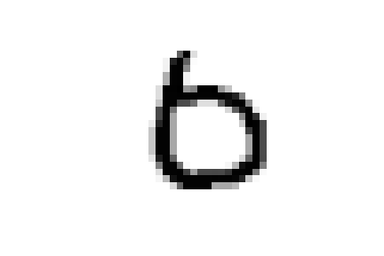
Here we are looking at a two-dimensional projection of our full dataset colour-coded according to the clusters identified (top) and then their original labels (bottom). We can see that the algorithm identified 6 different clusters that overlap very well with the labels. We see that most digits form a distinct, clearly defined group and end up forming their class in the hierarchy. For example '0_0' is mostly made up of digits representing 6, while '0_6' comprises 1. Looking at the bottom image we can see a certain degree of noise, certain digits do not go where they are expected to go, we see that in '0_3' there are some sevens, fours and a few twos (in grey, purple and green respectively). However, if we take a look at these specific cases we can see that this choice is completely justified.

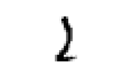
these samples are all closer to ones in the embedded space and could all be easily confused for ones Or again, we see a few nines and sixes in '0_5' which contains zeroes.

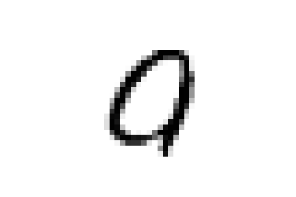
And as expected they are all characterized by wide circles as their most characterizing element.

There are however two major exceptions to our classes, '0_1' and '0_2' (in green and orange in the plot at the top) do not, for the most part, contain only a specific digit type, but are rather composite clusters.

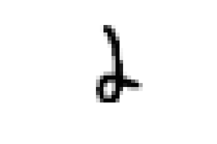
'0_1' is made up of a group of sevens, and overlapping clouds of nines and fours, while '0_2' contains threes, fives and eights. The commonality of their shapes (e.g. the latter are all characterized by a rounded stroke at the bottom) justifies their inclusion in a single class. However, the iterative search allows us to dig deeper and see if they separate at the next level, highlighting the importance of having a hierarchy of classes.

For the sake of brevity, we will only focus on '0_2'. At the next level, we see that eights (in yellow at the bottom) are gathered in their specific cluster '0_2_2' and so are part of the fives in '0_2_1'. However, the remaining samples, fives and threes again are all clumped together in '0_2_0'

Luckily for us, the final separation between threes and five is observed at the next level, within '0_2_0', where we see that all threes are found in '0_2_0_0' and the remaining five are in '0_2_0_1'.

Now we can ask ourselves, why samples representing the digit five were separated into two different classes found at different levels of the hierarchy. To answer this question we can compare the average shape of '0_2_1', the first class we encountered, that of '0_2_0_0' and also that of '0_2_0_1', which contains the threes and attracted part of the fives down its branch.

We can see that there are substantial structural differences between the two type of fives, with samples in '0_2_1' having a much more skewed shape, while those in '0_2_0_0' are rounder and considerably similar to threes for their bottom half, justifying their proximity.

The choice of t-SVD as an information filter, the use of density-based clustering or even the range and depth of the parameters space exploration, all contribute to this specific result. You can try changing these parameters, for example by running a more detailed search, and see how the hierarchy changes. You’ll see a few rearrangements, maybe more or fewer branches and levels in the tree of clusters, but overall, the shape of the main clusters and their composition won’t be mutated as long as your choices are appropriate for the dataset at hand.

Building a classifier

Finally, we can use this hierarchy of classes as a target for a prediction task. raccoon offers an implementation of a fuzzy k-nearest neighbour classifier, it just needs pickle files with the trained UMAP embeddings and consistency between the format of the training and the predicted data.

Note: if you are using MNIST for this tutorial, make sure to download some extra samples outside of the training dataset.

To run it, we import the kNN class, initialize it by passing the new data to assign, the original training set, its class assignment and path to the folder containing the pickle files. The results will be stored in the membership attribute.

from raccoon.utils.classification import KNN

rcknn=KNN(df_to_predict, df, cluster_membership, refpath=r'./raccoon_data', out_path=r'./')
rcknn.assign_membership()

new_membership = rcknn.membership

The classifier outputs a probability assignment, we impose a .5 cutoff to binarize the results and plot them in the following heatmap.

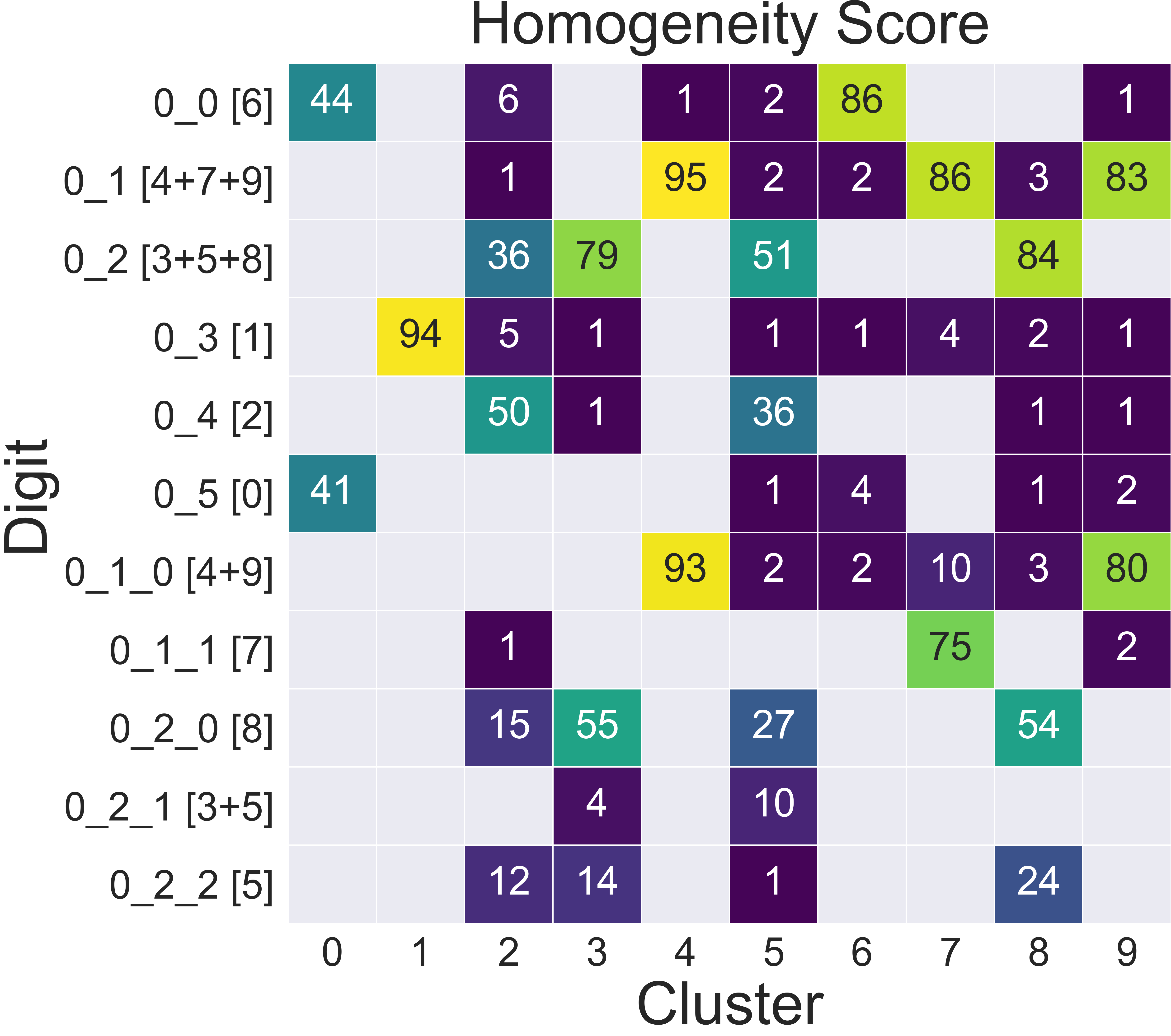
Here we are comparing the percentage of samples labelled according to a certain digit and where they are assigned in our hierarchy. To simplify we added in square brackets a clarification of their actual digit population content. We limit this comparison to the first levels, for clarity.

The classifier assigns most samples to the expected class, and more than that it can distinguish subclasses within each digit group that we identified deeper in the hierarchy. However, since this classification is based on the unsupervised classes, borderline samples as those shown before will be assigned to the class that is most similar in the pixels space, rather than the labels that came with the dataset. There is value in this, as it allows us to get rid of possible errors or inaccuracies in the labelling. These classes fit closely the shape of the data and can be used as target classes for considerably more accurate classification tools (e.g. neural nets).